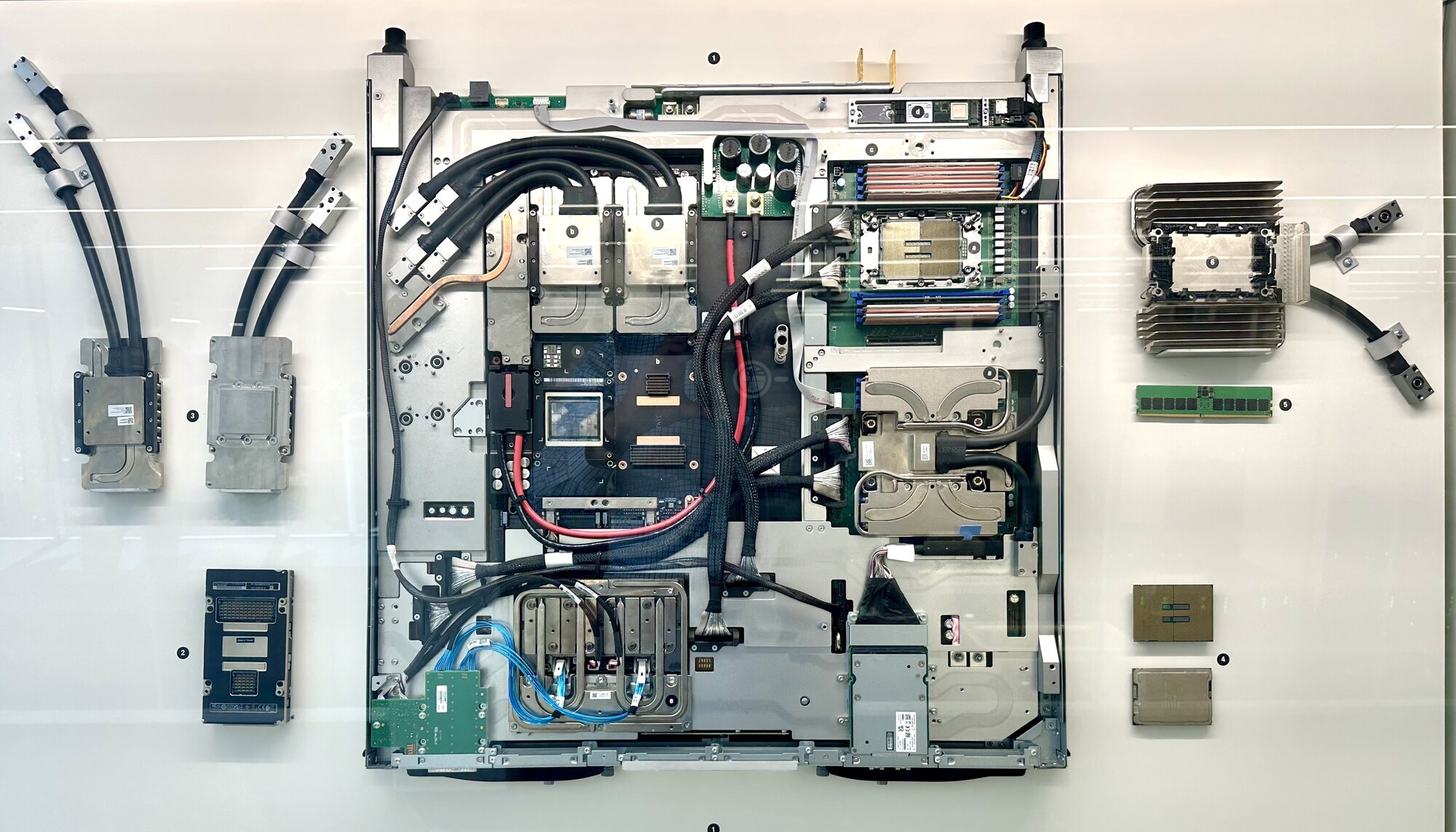
Scientific computing
Scientific Computing
Simulations of cardiac function at the organ scale — electrophysiology, deformation, hemodynamics — are computationally demanding. Electrophysiology needs a fine spatio-temporal mesh to resolve the fast, steep depolarization wavefront (under 1 ms, under 1 mm); the non-linear equations of tissue deformation need less resolution, but are correspondingly more expensive to solve.
Clinical use compounds the cost: personalizing a model for diagnosis [Niederer et al, 2010], disease stratification [Arevalo et al, 2016], or therapy planning requires many forward simulations inside an optimization loop that re-parameterizes the model until it matches clinical data. We address this with efficient numerical methods that exploit high performance computing hardware, and with model formulations that need less resolution in the first place.
Numerical Methods and Algorithms
Finite Element Discretization
Patient-specific anatomical models are discretized with the finite element method (FEM) on unstructured, boundary-fitted grids (see image-based mesh generation). The same mesh serves both the electrophysiology and the nonlinear elasticity equations, so there is no need to map data between separate electrical and mechanical grids.
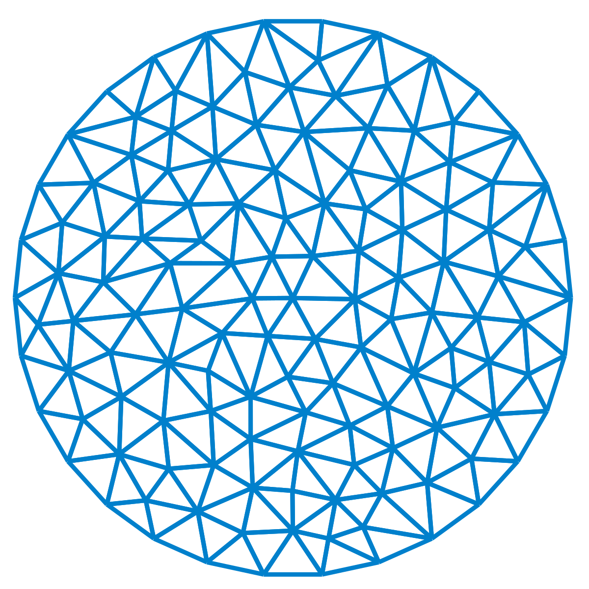
Figure 1: Finite element discretization
Domain Decomposition
The sparse linear systems produced by FEM discretization are partitioned across compute nodes for parallel solution. We compare our own non-overlapping partitioning scheme, pt, against the widely used overlapping partitioning of PETSc — trading fragmented interface rows for a leaner memory footprint and less inter-node communication [Neic et al, 2012].
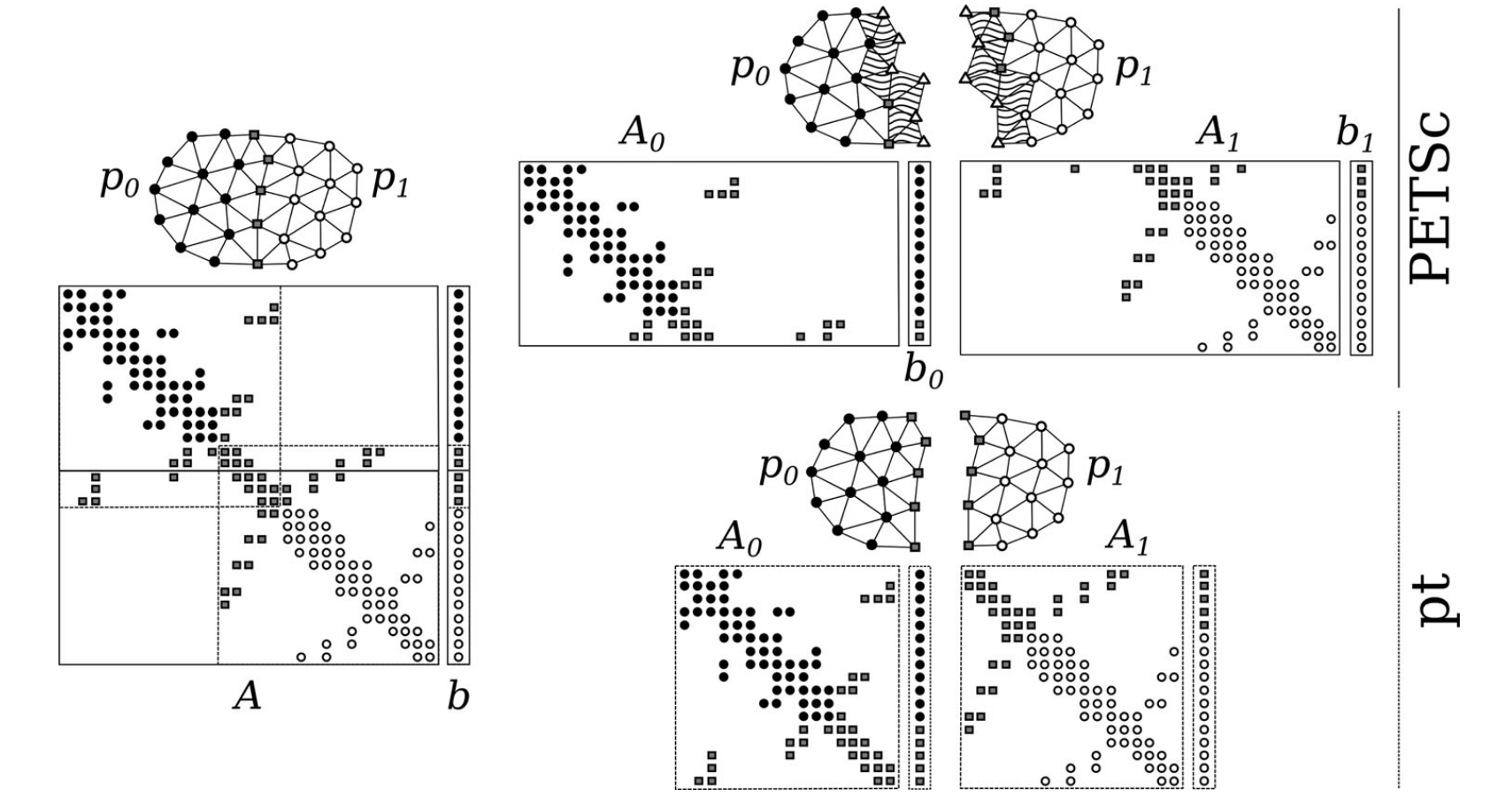
Figure 2: Domain-decomposition parallelization strategies
Scalable Solvers for Nonlinear Elasticity
Solving Cauchy’s equation of motion at high spatial resolution produces very large, ill-conditioned nonlinear systems. We developed a novel algebraic multigrid (AMG) preconditioner for an iterative Krylov solver, designed specifically for favorable strong scaling of both the setup and the solution phase [Augustin et al, 2016]. On whole heart electromechanics models of up to 184.6 million tetrahedral elements, it scales efficiently to 8192 compute cores — see strong scaling below.
High Performance Computing
Strong Scaling
Increasing the number of compute cores to reduce execution time is strong scaling. It is limited by the ratio of local compute work (volume) to communication cost (surface): as cores are added, the volume-to-surface ratio shrinks until communication starts to dominate — the limit of strong scalability — beyond which adding cores no longer helps, and can even hurt, execution time. At very high core counts, I/O cost grows for the same reason.
Optimizing strong scaling therefore means distributing workload and communication evenly, decomposing the domain into volumes with minimal surface area, and hiding the cost of I/O. The two figures below show this in practice, in two of our simulation codes.
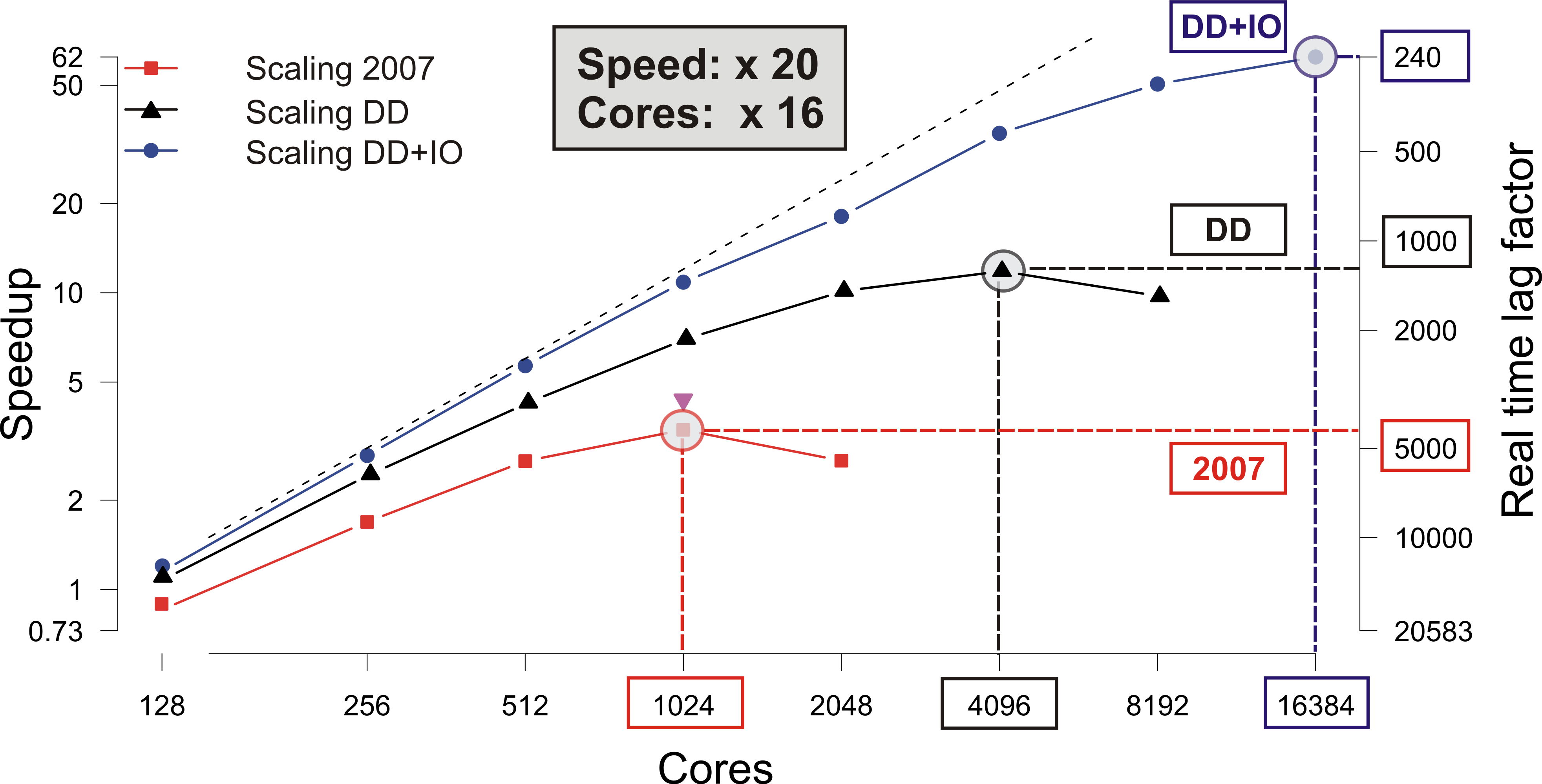
Figure 3: Strong scaling from improved domain decomposition and I/O
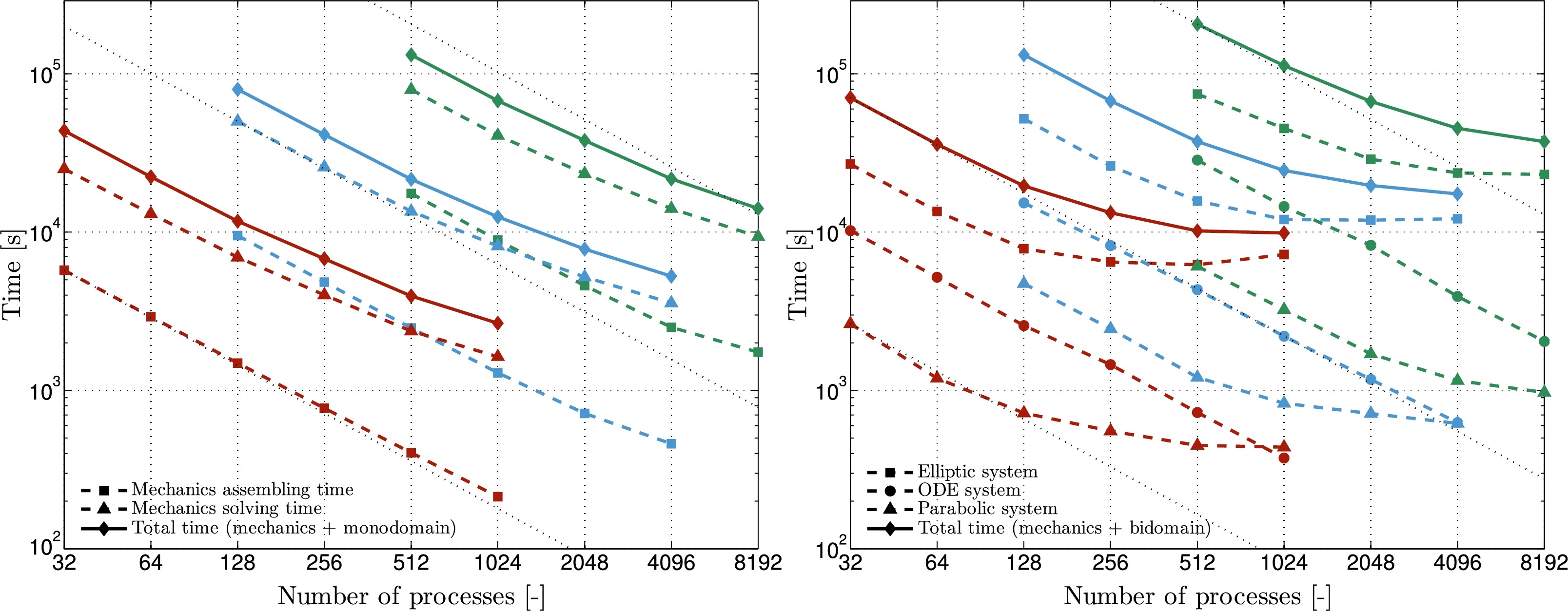
Figure 4: Strong scaling of the AMG-preconditioned EP/electromechanics solver
Use of Accelerators
GPUs are well suited to the large, sparse linear systems that arise from bidomain simulations. Porting our simulator to multi-GPU execution required only minor changes to the existing CPU code base: benchmarks on a state-of-the-art rabbit ventricle model showed bidomain simulations sped up by a factor of 11.8–16.3× on 6–20 GPUs versus the same number of CPU cores — matching the fastest 20-GPU run took 476 CPU cores on a national supercomputing facility [Neic et al, 2012].