The Cardiac Bidomain Equation

Cardiac tissue at a microscopic size scale is a discrete structure. From an electrical point of view the most important building block are myocytes, in which the sarcolemmnal membrane separates the intracellular space inside the myocyte from the interstitial space in between myocytes. The intracellular spaces of adjacent myocytes are tightly coupled by gap junctions, therefore cardiac tissue can be considered a functional syncytium. Electrical behavior of cardiac tissue when observed from a more macroscopic point of view can be considered a continuum.

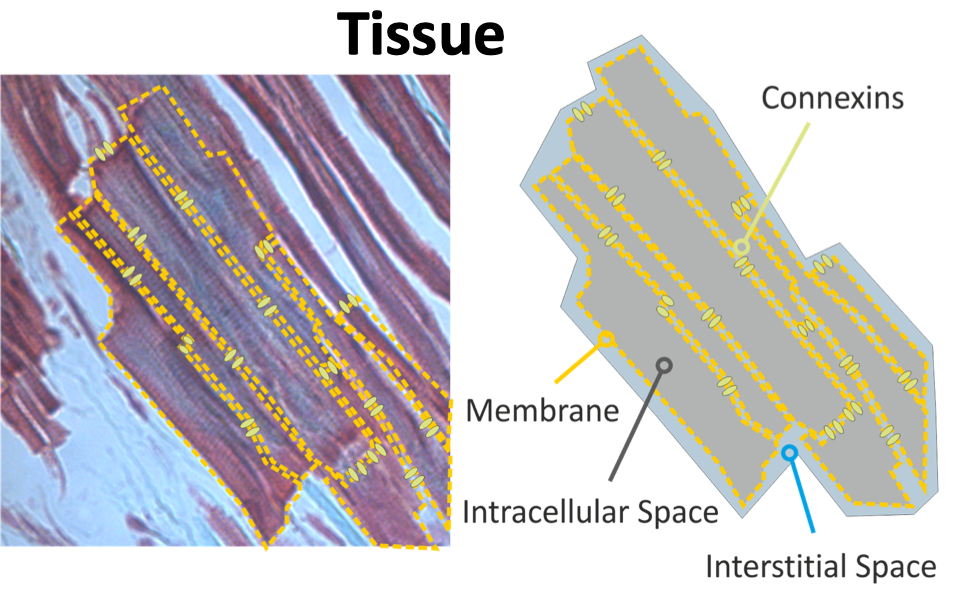
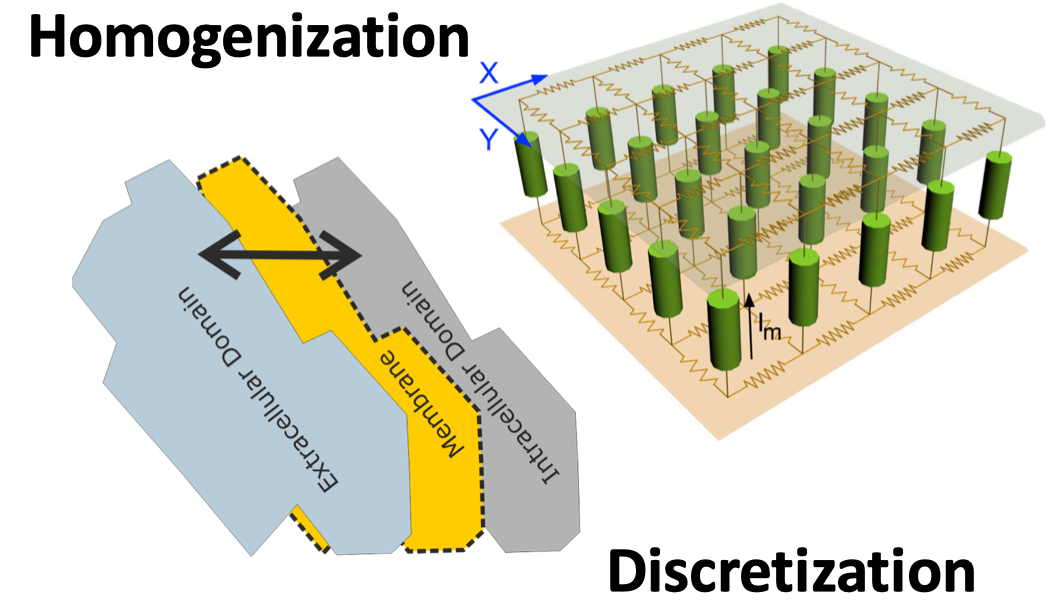
Figure 1: Discrete nature of cardiac tissue and its representation as a continuum in a homogenized model

Tissue: Cardiac tissue consists of discrete myocytes which are interconnected via gap junctions. Homogenization: Discrete structures in the intracellular and extracellular spaces within the myocardium are homogenized to arrive at a continuum representation, the electrical properties at the discrete microscopic scale and at the continuous macroscopic scale match. Both homogenized domains are overlapped, separated by a membrane at each point in space (interpenetrating domains). Spatial discretization: Discrete representation of both conductive domains, intra- and extracellular, and the membrane.

In terms of modeling cardiac electrophysiology at the tissue scale continuum representations prevail. While discrete models representing tissue as interconnected myocytes are, in principle, feasible and have been reported in the literature, as the heart is composed of around 5 billion myocytes such models are computationally extremely expensive, limiting their application to smaller tissue specimens. For larger tissue specimens up to the whole heart the macroscopic cardiac bidomain equations are considered the most complete mathematical model describing the spread of cardiac electrical activity. The bidomain model can be derived based on geometric assumptions on cellular structures through a homogenization procedure, yielding a continuum formulation where tissue properties are taken into account in an averaged sense. The domains of interest - intracellular and extracellular - are preserved in the formulation. The membrane separates intracellular from interstitial space. Both spaces - intracellular and extracellular - interpenetrate each other and co-exist everywhere. Current can flow from one space to the other by crossing the separating membrane. Charge conservation in both domains yields then the following equations:

Equation 1: Cardiac Bidomain Model

$$ \begin{align} \nabla \cdot \sigma_{\rm i} \nabla \phi_{\rm i} &= \beta I_{\rm m} \\ \nabla \cdot \sigma_{\rm e} \nabla \phi_{\rm e} &= -\beta I_{\rm m} + I_{\rm } \end{align} $$ where $\beta$ is the surface area of membrane contained within a unit volume, $I_{\mathrm{e}}$ is an extracellular current density, specified on a per volume basis, which serves as a stimulus to initiate propagation, ${\phi }_{\mathrm{X}}$ and ${\sigma }_{\mathrm{X}}$ are the electrical potential and homogenized conductivity in the domain $\mathrm{X}$ respectively, where $\mathrm{X}$ is $\mathrm{i}$ or $\mathrm{e}$ for intracellular or extracellular. The conductivity tensors describe the orthotropic eigendirections of the tissue at a given location, $\mathbf{x}$, and are constructed as $$ \sigma_{\mathrm{X}} = \sigma_{\mathrm f, \mathrm X} \, \mathbf{f} \otimes \mathbf{f} + \sigma_{\mathrm s, \mathrm X} \mathbf{s} \otimes \mathbf{s} + \sigma_{\mathrm n, \mathrm X} \mathbf{n} \otimes \mathbf{n}, $$ where ${\sigma }_{\mathrm{f},\mathrm{X}}$, ${\sigma }_{\mathrm{s},\mathrm{X}}$ and ${\sigma }_{\mathrm{n},\mathrm{X}}$ are conductivities of the domain $\mathrm{X}$ along the local eigenaxes, $\mathbf{f}$, along the prevailing myocyte orientation referred to as fiber orientation, perpendicular to the fiber orientation but within a sheet, $\mathbf{s}$, and the sheet normal direction, $\mathbf{n}$. The transmembrane voltage $V_m$ is given as the difference between intra- and extracellular potential $$ V_{\rm{m}} = \phi_{\rm{i}} - \phi_{\rm{e}} $$ and the transmembrane current $I_{\mathrm{m}}$ is given by $$ \begin{align} I_{\rm{m}} &= C_{\rm{m}} \frac{\partial V_{\rm{m}}}{\partial t} + I_{\rm{ion}}(V_{\rm{m}},\boldsymbol{\eta}) \\ \frac{\partial \boldsymbol{\eta}}{\partial t} &= f(V_{\rm m}, \boldsymbol{\eta}) \end{align} $$ where $C_{\mathrm{m}}$ is the membrane capacitance, and $\mathit{\eta }$ is a vector of state variables describing the cellular dynamics governed by gating mechanisms and ion fluxes. That is, the transmembrane current $I_{\mathrm{m}}$ consists of a capacitive current $I_{\mathrm{c}}$ and a current due to ions crossing the membrane, $I_{\mathrm{ion}}$.

The fast upstroke of the action potential lasting less than 1 ms translates into steep depolarization wave fronts in space of a spatial extent of less than 1 mm. This spatio-temporal dynamics render solving the bidomain equations computationally expensive since high spatio-temporal resolutions are needed to achieve sufficient accuracy. Typically, spatio-temporal resolutions of 50 μs and 250 μm or finer are used as shown in standard electrophysiology verification benchmarks.

The Eikonal Equation

In the early nineties, the eikonal model has been proposed as an efficient way of computing arrival times of depolarization wavefronts in the myocardium, and its potential limitations have been studied extensively [Franzone and Rovida, 1990], [Keener, 1991], [Franzone et al., 1998]. Wavefront arrival times based on the eikonal model have also been used to prescribe the spatio-temporal evolution of the transmembrane voltage to predict extracellular potentials and electrograms [Franzone et al., 1993], [Franzone et al., 1998], [Franzone et al., 2000].

Equation 2: Eikonal Model

In the eikonal model, wavefront arrival times $t_{\mathrm{a}}$ in the myocardium $\Omega$ are described based on a spatially heterogeneous orthotropic velocity function encoded as $\mathbf{V}\left(\mathrm{x}\right)$ and initial activations $t_0$ at locations $\Gamma$. The eikonal equation is of the form $$ \left\{ \begin{array}{rcll} \sqrt{\nabla t_{\rm a}^\top \, \mathbf{V} \, \nabla t_{\rm a}} & = & 1 \qquad & \text{in } \Omega \\ t_{\rm a} & = & t_0 & \text{in } \Gamma \end{array} \right. \label{eq:_eikonal} $$ where $\Omega$ is the myocardium and $t_{\mathrm{a}}$ is a positive function describing the wavefront arrival time at location $\mathrm{x}$. The symmetric positive definite $3\times 3$ tensor $\mathbf{V}\left(\mathbf{x}\right)$ holds the squared velocities $\left(v_{\mathrm{f}}\right(\mathbf{x}),v_{\mathrm{s}}(\mathbf{x}),v_{\mathrm{n}}(\mathbf{x}\left)\right)$ associated to $\left(\mathbf{f}\right(\mathbf{x}),\mathbf{s}(\mathbf{x}),\mathbf{n}(\mathbf{x}\left)\right)$, respectively the longitudinal, transversal and normal fiber directions: $$ \boldsymbol{V} := v_{\rm f}^2 \mathbf{f} \, \mathbf{f}^\top + v_{\rm s}^2 \mathbf{s} \, \mathbf{s}^\top + v_{\rm n}^2 \mathbf{n} \, \mathbf{n}^\top $$ This definition is analogous to the that of the conductivity tensors ${\sigma }_{\mathrm{X}}$ above in bidomain equation, and since $\mathbf{V}\left(\mathbf{x}\right)$ and ${\mathbf{\sigma }}_{\mathbf{i}}\left(\mathbf{x}\right)$ are based on the same orthotropic fiber and sheet arrangement $(\mathbf{f},\mathbf{s},\mathbf{n})$ it follows that the velocities $(v_{\mathrm{f}},v_{\mathrm{s}},v_{\mathrm{n}})$ and the conductivities ${\sigma }_{\mathrm{f},\mathrm{X}}$, ${\sigma }_{\mathrm{s},\mathrm{X}}$ and ${\sigma }_{\mathrm{n},\mathrm{X}}$ forming ${\mathbf{\sigma }}_{\mathrm{X}}$ must be proportionally coupled. While conductivities and velocities for a uniformly propagating planar depolarization wave front are proportionally related by $$ v_{\rm X} \propto \sqrt{\frac{\sigma_{\rm{m,X}}}{\beta}} $$ with ${\sigma }_{\mathrm{m,X}}$ being twice the harmonic mean conductivity tensor given as $$ \sigma_{\rm{m,X}} = \frac{\sigma_{\rm{i,X}} \, \sigma_{\rm{e,X}}}{\sigma_{\rm{i,X}} + \sigma_{\rm{e,X}}} $$ fitting of conductivities to match a desired conduction velocity is a non-trivial task since simulated velocities are also influenced by a number of technical factors such as spatio-temporal discretization, chosen element type or integration rules. Methods for automated fitting have been discussed elsewhere [Mendonca Costa et al. 2013].