Cardiovascular Hemodynamics
Cardiac and Vascular Blood Flow
The Navier-Stokes equations, named after Claude-Louis Navier and George Gabriel Stokes, describe the motion of viscous fluid substances. The equations are derived from the basic principles of continuity of mass, momentum, and energy. $$ \frac{\partial}{\partial t} (\rho u_{i}) + \frac{\partial}{\partial x_{j}} (\rho u_{i} u_{j} + p \delta_{ij} - \tau_{ji} ) = 0 $$ where in case of an Newtonian fluid $$ \tau_{ij} = 2\mu S_{ij}^{*} $$ and $$ S_{ij}^{*} = \frac{1}{2} \left( \frac{\partial u_{i}}{\partial x_{j}} + \frac{\partial u_{j}}{\partial x_{i}} \right) - \frac{1}{3} \frac{\partial u_{k}}{\partial x_{k}} \delta_{ij}. $$
Reduced-order models are based on simplified representations of the components of the cardiovascular system and contribute to the understanding of circulatory physiology. Furthermore, they require a reduced computational cost compared to higher-dimensional computational fluid dynamics methods.
Lumped Circulatory Models
Zero-dimensional (lumped) models are based on a hydraulic-electrical analogue and represent the simplest way to analyse global haemodynamic interactions among the cardiovascular organs. However, they are unable to describe nonlinearities such as convective acceleration terms and the nonlinear relationship between pressure and cross-sectional area in a vessel. Numerous zero-dimensional models of the systemic vasculature have been described ranging from the simple two element Windkessel model [Frank, 1899] to more complex models such as the Guyton model [Guyton et al., 1972] and can be classified into mono- and multi-compartment models. Mono-compartment models desribe the cardiovascular system through a single combination of resistance, compliance and inductance. A schematic representation of the widely used three-element Winkessel model [Westerhof et al., 1971] is shown below, featuring the two element Windkessel (total arterial resistance (R) and total arterial compliance (C) in parallel) in series to aortic impedance (Z), which can be formulated as the following ODE: $$ \frac{dp}{dt} = \left( \frac{1}{C}+\frac{Z}{RC} \right) q + Z \frac{dq}{dt} - \frac{1}{RC} p $$ where \(q\) is the flow across the aortic valve and \(p\) the pressure in the aorta ascendens.
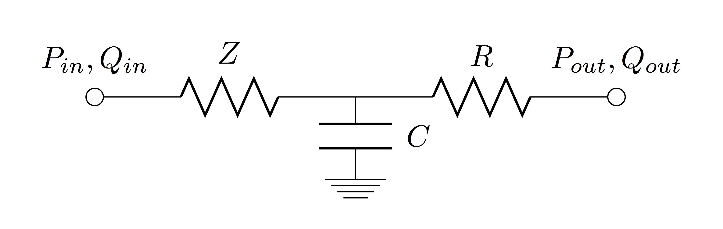
This model can be preferred over its extensions, namely the four element Winkessel models (with inductance (L) in parallel or series to Z), as it accurately describes pressure-flow relations in the aorta ascendens while only using physiologically meaningful parameters. An additional advantage is the rather simple ventriculo-arterial coupling when using the three element Windkessel model. In multi-compartment models the vasculature is divided into several segments, each having there own characteristics.
One-dimensional Circulatory Models
One-dimensional (1D) blood flow models enable an efficient representation of the effects of pulse wave transmission and reflection in the circulation. In particular, 1D models may be preferred over 0D models when local vascular changes or distributed properties and their impact on central pressure waveforms are studied and when the effects of pulse wave transmission on the circulation are under investigation. For example, vessel branching, change of vessel properties (tapering, stenoses, collapse, stents) and nonlinear pressure-area relationships can be included in such models. Therefore, they are particularly suitable to simulate blood flow in the aorta and the major arteries and veins. Numerous models have been proposed, based on different formulations and discretization approaches [Formaggia et al., 2003], [Mynard et al., 2008], [Müller and Toro, 2013], [Blanco et al., 2014]. A recent benchmark study on six commonly used numerical schemes for 1D blood flow modeling [Boileau et al., 2015] showed a good agreement among these schemes and their capability to capture the main characteristics of flow and pressure waveforms in the large arteries.
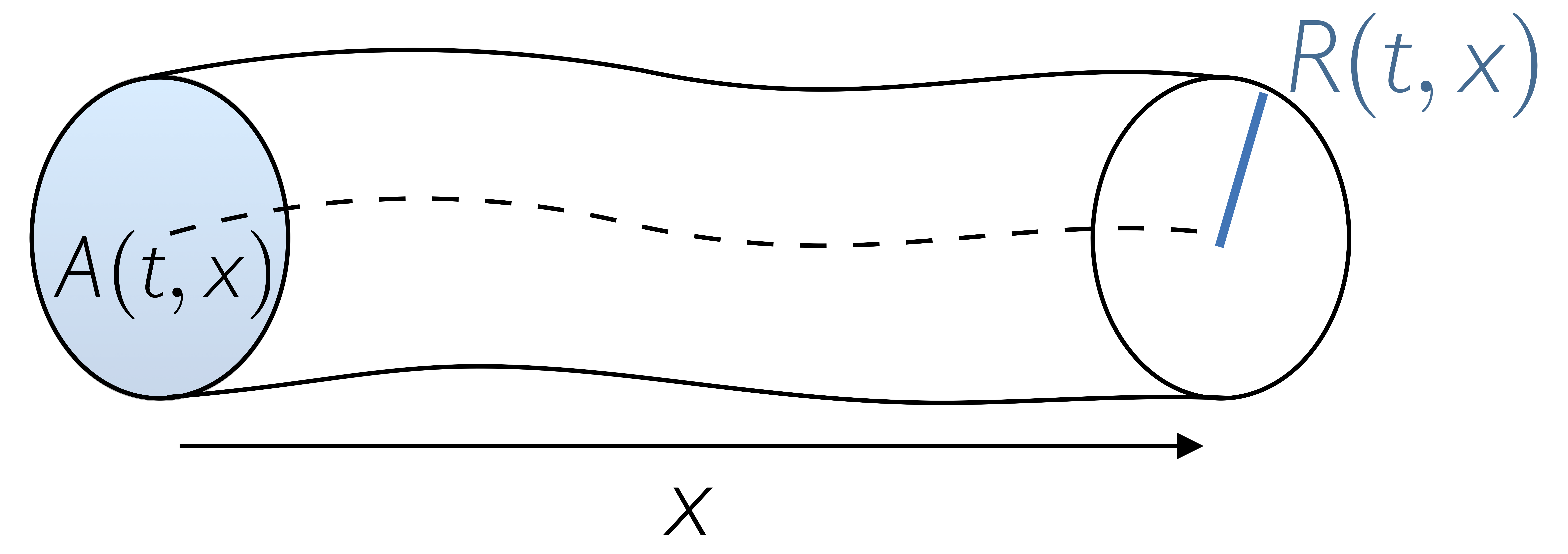
The one-dimensional equations of blood flow are derived by integrating the Navier-Stokes equations of a generic section of the tube, after assuming axisymmetric flow and a cylidrical tube. In more detail, if we assume a flat velocity profile, we obtain the system $$ \left\{ \begin{array}{l} \displaystyle \frac{\partial A}{\partial t}+\frac{\partial (Au)}{\partial x}=0 \\[6pt] \displaystyle \frac{\partial u}{\partial t} + u\frac{\partial u}{\partial x}+\frac{1}{\rho} \frac{\partial P}{\partial x}= \frac{f}{ \rho A}, \end{array} \right. \label{eq:1D_BF_Au} $$ where \(A(x,t) \) is the cross-sectional area of the lumen, \(u(x,t) \) is the average axial velocity and \(P(x,t)\) is the average internal pressure over the cross-section. For a constant velocity profile satisfying no-slip condition, the friction force per unit length is \(f(x,t)= -\eta u(x,t) \), where \(\eta \) is a coefficient depending on the blood viscosity and the average axial velocity. As the system of equations is composed by two equations and three unknowns \( (A,u,P) \), a closure condition is needed, namely the so-called tube law: $$ P(x,t)=P_{ext}(x,t)+K\,\phi\bigl(A(x,t),A_0(x)\bigr)+G \,\Psi\bigl(A(x,t)\bigr), \label{tubelaw} $$ where \(K \) and \(G \) are parameters depending on the wall stiffness and the viscosity, respectively. A simple, purely elastic tube law consists in defining $$ \phi = \frac{\sqrt{A}- \sqrt{A_0}}{A_0}, \quad K = \frac{4}{3}\sqrt{\pi}Eh,\quad \text{and}\quad \Psi =0, $$ with \(E \) the Young modulus and \(h\) the wall thickness of the vessel. A more complex tube law is obtained when visco-elastic effects are considered, e.g. by setting $$ \Psi = \frac{1}{A_0\sqrt{A}} \frac{\partial A}{\partial t}, \quad G = \frac{2}{3} \sqrt{\pi}\varphi h, $$ with \( \varphi(x)\) the wall viscosity.